Section 11.2: Inference about Two Means
Objectives
By the end of this lesson, you will be able to...
- distinguish between independent and dependent samples
- test hypotheses regarding matched-pairs data
- construct and interpret confidence intervals about the population mean difference of matched-pairs data
For a quick overview of this section, watch this short video summary:
In the next two sections, we'll focus on the relationship between two means. Before we begin, we need to discuss the two possible situations.
Independent vs. Dependent Samples
In general, there are two possible situations regarding two population means. Consider the following examples:
Example 1
Problem: Suppose we measure the thickness of plaque (mm) in the carotid artery of 10 randomly selected patients with mild atherosclerotic disease. Two measurements are taken, thickness before treatment with Vitamin E (baseline) and after two years of taking Vitamin E daily. (Source: UCLA Dept. of Statistics)
Discussion: In this example, we would be comparing the mean plaque thickness before Vitamin E with the mean thickness after - so the same 10 patients would be in the sample "before" and the sample "after". When the individuals slected are paired in this manner, we call the samples dependent.
Example 2
Problem: Nine observations of surface soil pH were made at two different locations. Does the data suggest that the true mean soil pH values differ for the two locations? (Source: UCLA Dept. of Statistics)
Discussion: Unlike in Example 1, the samples in this example are completely unrelated (two different locations). In examples like this, where the indivuaduals selected have no relation to each other, we call the samples independent.
In general, two samples are dependent if the individuals in one sample determine the individuals in the other sample. (i.e. matched-pair design) Two samples are independent when the individuals in one sample do not determine the individuals in the other sample. (i.e. completely randomized)
This will be very important as we progress, because we will need to distinguish between whether the samples are dependent or independent, because the statistical methods will be very different.
The Difference of Two Independent Means
In 2005, Larry Summers, then President of Harvard, gave a speech at the NBER Conference on Diversifying the Science and Engineering Workforce. In that speech, he made some very controversial remarks regarding differences in the genders. In particular,
It does appear that on many, many different human attributes-height, weight, propensity for criminality, overall IQ, mathematical ability, scientific ability-there is relatively clear evidence that whatever the difference in means-which can be debated-there is a difference in the standard deviation, and variability of a male and a female population.
Suppose we wanted to do a comparison between the genders. In Section 11.2, we looked at comparing two means with matched-pairs data - dependent samples. What if there isn't a relationship between the two samples? We certainly can't pair them up then, and find the mean difference. What we need to anlyze instead is the difference of two means. First, we need to know something about it's distribution.
The Distribution of the Difference of Two Means, d
Suppose a simple random sample of size n1 is taken from a population with unknown mean μ1 and unknown standard deviation σ1. In addition, a simple random sample of size n2 is taken from a second population with unknown mean μ2 and unknown standard deviation σ2. If the two populations are normally distributed or the sample sizes are sufficiently large (n1, n2≥30), then

approximately* follows the t-distribution with the smaller of n1-1 or n2-1 degrees of freedom.
Note: There is no exact method for comparing two means with unequal populations, but this statistic is a close approximation. It is known as Welch's approximate t, in honor of English statistician Bernard Lewis Welch (1911-1989).
Now that we have the distribution of the difference between two means, we can perform statistic inference (hypothesis testing and confidence intervals).
Performing a Hypothesis Test Regarding the Difference Between Two Independent Means
Step 1: State the null and alternative hypotheses.
| Two-Tailed H0: μ1-μ2 = 0 H1: μ1-μ2 ≠ 0 |
Left-Tailed H0: μ1-μ2 = 0 H1: μ1-μ2 < 0 |
Right-Tailed H0: μ1-μ2 = 0 H1: μ1-μ2 > 0 |
Step 2: Decide on a level of significance, α.
Step 3: Compute the test statistic,  .
.
Step 4: Determine the P-value.
Step 5: Reject the null hypothesis if the P-value is less than the level of significance, α.
Step 6: State the conclusion.
Hypothesis Testing Regarding μ1-μ2 Using StatCrunch
The results should appear. |
A note about the difference between the means: As with the previous section, it's often difficult for students to choose which mean to place first. Again - it doesn't matter! The important thing is to note clearly in your work what the order is, and then to construct your alternative hypothesis accordingly.
Example 1
Problem: Suppose we wish to test whether there is a difference in the performances of men and women in mathematics. An ECC instructor collects exam scores from 2 semesters worth of Beginning Algebra students, shown below by gender.
| Women | Men | |||||||||||||
| 94 | 90 | 96 | 73 | 71 | 75 | 52 | 77 | 57 | 79 | 65 | 68 | 65 | 55 | |
| 86 | 93 | 86 | 50 | 30 | 46 | 36 | 72 | 66 | 29 | 69 | 85 | 82 | 43 | |
| 82 | 55 | 75 | 47 | 80 | 92 | 56 | 60 | 64 | 82 | 91 | 51 | 60 | 76 | |
| 43 | 77 | 63 | 76 | 67 | 99 | 93 | 43 | 82 | 87 | 32 | 71 | 77 | 77 | |
| 75 | 90 | 92 | 88 | 76 | 61 | 77 | 79 | 97 | 56 | |||||
| 49 | 67 | 81 | 89 | 88 | 42 | 51 | ||||||||
| 58 | 98 | 46 | 96 | 90 | 46 | 50 | ||||||||
| 67 | 83 | 85 | ||||||||||||
Click here to see the data in CSV format.
Is there enough evidence at the 5% level of significance to support the claim that men and women perform differently in this class?
Solution:
First, we need to make sure that neither sample contains outliers. (We do have sample sizes of at least 30, so we don't need to check to see if they come from normally distributed populations.)
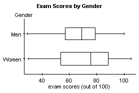
We can see that neither sample contains outliers, so we are free to continue.
Step 1:
In this case, since we're only testing whether the means are different,
the order doesn't matter at all. It's easiest to simply take the two in
the order we receive them, so
μ1 = μW (women), and μ2 = μM (men).
H0: μW-μM = 0
H1: μW-μM ≠ 0
Step 2: α = 0.05 (given)
Step 3: (we'll use StatCrunch)
Step 4: Using StatCrunch:
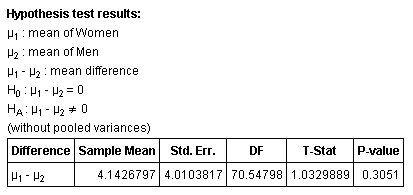
Step 5: Since the P-value > α, we do not reject the null hypothesis.
Step 6: Based on these results, it would appear that there is not enough evidence (very little, in fact) to support the claim that men and women perform differently in Beginning Algebra.
It should be noted that larger sample sizes will most likely show a statistically significant difference, though the difference may not have any practical meaning.
One final note, you may wonder what the "pooled variances" is referring to, and why we don't use it. By not pooling the variances, we are assuming that the population variances are unequal. There is a test for equal variances (we'll cover it in Section 11.4), but like the earlier tests concerning standard deviations, the distributions must be normal.
The issue here is that the test for equal variances is very senstive - so even small differences will be statistically signifcant. It's generally safer to just assume the variances are different, as the two tests (assuming equal variances by pooling or by not assuming equal variances), so going through the test for variances is not particularly valuable.
Confidence Intervals about the Difference Between Two Means
Since the distribution of ![]() follows the t-distribution, we can also create a confidence interval for the difference between two population means.
follows the t-distribution, we can also create a confidence interval for the difference between two population means.
In general, a (1-α)100% confidence interval for μ1-μ2is

where ![]() is computed with min{n1-1, n2-1} degrees of freedom.
is computed with min{n1-1, n2-1} degrees of freedom.
Note: The sample sizes must be large (n1,n2≥30) with no outliers or the populations must be normally distributed.
Confidence Intervals About μ1-μ2 Using StatCrunch
The results should appear. |
Example 2
Problem: Consider the data comparing men and women from Example 1.
| Women | Men | |||||||||||||
| 94 | 90 | 96 | 73 | 71 | 75 | 52 | 77 | 57 | 79 | 65 | 68 | 65 | 55 | |
| 86 | 93 | 86 | 50 | 30 | 46 | 36 | 72 | 66 | 29 | 69 | 85 | 82 | 43 | |
| 82 | 55 | 75 | 47 | 80 | 92 | 56 | 60 | 64 | 82 | 91 | 51 | 60 | 76 | |
| 43 | 77 | 63 | 76 | 67 | 99 | 93 | 43 | 82 | 87 | 32 | 71 | 77 | 77 | |
| 75 | 90 | 92 | 88 | 76 | 61 | 77 | 79 | 97 | 56 | |||||
| 49 | 67 | 81 | 89 | 88 | 42 | 51 | ||||||||
| 58 | 98 | 46 | 96 | 90 | 46 | 50 | ||||||||
| 67 | 83 | 85 | ||||||||||||
Find a 90% confidence interval for the population mean difference.
Solution: From Example 1, we know that neither sample contains outliers, so we can find the confidence interval.
Using StatCrunch:
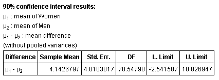
So we can say that we're 90% confident that the difference between the two means is between -2.5 and 10.8.
The Difference, d
When considering dependent samples, we analyze the difference, d, in each matched pair. For example, suppose we consider the thickness of plaque (mm) in the carotid artery, referenced in Example 1. If an individual had a maximal thickness of 0.92mm before the Vitamin E treatment, and 0.95mm after the treatment, the difference, d, for that individual would be
d = 0.95 - 0.92 = 0.03mm
So in general, for this experiment, we would define the difference, d, to be:
d = thickness after Vit. E treatment - thickness before treatment
Before we can perform any inferential statistics, we need to know the distribution of d.
The Distribution of the Difference, d
Suppose the following are true concerning a sample:
- the sample is obtained using simple random sampling, and
- the sample data are matched pairs, and
- the sample has no outliers and the population from which the sample is drawn is normally distributed, or the sample size is large (n≥30).
Then the test statistic
![]()
follows the t-distribution with n-1 degrees of freedom.
With that in mind, we can now perform statistical inference like hypothesis tests and confidence intervals. We'll start with hypothesis tests, and follow the same steps we did when we were analyzing the population mean, when σ was unknown.
A note about the difference, d: Many students find it confusing how to determine which value should go first when setting up the difference. In reality, it doesn't matter! The important thing is to note clearly in your work how d is set up, and then to construct your alternative hypothesis accordingly.
Performing a Hypothesis Test Regarding d
Step 1: State the null and alternative hypotheses.
| Two-Tailed H0: μd = 0 H1: μd ≠ 0 |
Left-Tailed H0: μd = 0 H1: μd < 0 |
Right-Tailed H0: μd = 0 H1: μd > 0 |
Step 2: Decide on a level of significance, α.
Step 3: Compute the test statistic, ![]() .
.
Step 4: Determine the P-value.
Step 5: Reject the null hypothesis if the P-value is less than the level of significance, α.
Step 6: State the conclusion.
Hypothesis Testing Regarding d Using StatCrunch
The results should appear. |
Example 3
Problem: Suppose we want to determine if a diet drug is effective. To determine it's effectiveness, we randomly select 10 volunteers, and measure their weight before the diet drug treatment, and again one month later. The results are shown below.
| A | B | C | D | E | F | G | H | I | J | |
| Before | 190 | 211 | 198 | 203 | 262 | 224 | 251 | 238 | 219 | 255 |
| After | 184 | 204 | 197 | 208 | 246 | 221 | 256 | 225 | 211 | 243 |
Is there evidence to support the company's claim that the diet drug does cause weight loss at the 5% level of significance?
Solution:
First, we need to calculate the differences. It's important to always write down which direction you want to define the difference, d. In this case, we'll use:
d = Before - After
| A | B | C | D | E | F | G | H | I | J | |
| Before | 190 | 211 | 198 | 203 | 262 | 224 | 251 | 238 | 219 | 255 |
| After | 184 | 204 | 197 | 208 | 246 | 221 | 256 | 225 | 211 | 243 |
| Difference | 6 | 7 | 1 | -5 | 16 | 3 | -5 | 13 | 8 | 12 |
We need to then determine if the differences are normally distributed, since our sample size is less than 30.
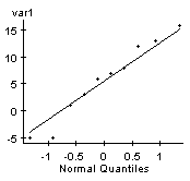
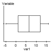
We can see that the Q-Q plot is fairly linear and the boxplot shows no outliers, so it's reasonable to say that the differences are normally distributed.
Step 1:
H0: μd = 0
H1: μd > 0
(Since the company wants to show that the average weight loss is positive.)
Step 2: α = 0.05 (given)
Step 3: (we'll use StatCrunch)
Step 4: Using StatCrunch:
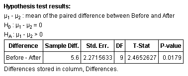
Step 5: Since the P-value < α, we reject the null hypothesis.
Step 6: Based on these results, it would appear that there is enough evidence to support the claim that the drug causes weight loss.
Note: If we had first set up the difference as d = After - Before, the alternative hypothesis would then be H1: μd < 0 (since the company claims the "after" is less than the "before").
Confidence Intervals about the Mean Difference
Since the distribution of ![]() follows the t-distribution, we can also create a confidence interval for the population mean difference.
follows the t-distribution, we can also create a confidence interval for the population mean difference.
In general, a (1-α)100% confidence interval for μdis
![]()
where ![]() is computed with n-1 degrees of freedom.
is computed with n-1 degrees of freedom.
Note: The sample size must be large (n≥30) with no outliers or the population must be normally distributed.
Confidence Intervals About μd Using StatCrunch
The results should appear. |
Example 4
Problem: Consider the weight loss data from Example 3.
| A | B | C | D | E | F | G | H | I | J | |
| Before | 190 | 211 | 198 | 203 | 262 | 224 | 251 | 238 | 219 | 255 |
| After | 184 | 204 | 197 | 208 | 246 | 221 | 256 | 225 | 211 | 243 |
Find a 90% confidence interval for the population mean difference.
Solution:
From Example 3, we know that the differences are normally distributed with no outliers, so we can find the confidence interval.
d = Before - After
| A | B | C | D | E | F | G | H | I | J | |
| Before | 190 | 211 | 198 | 203 | 262 | 224 | 251 | 238 | 219 | 255 |
| After | 184 | 204 | 197 | 208 | 246 | 221 | 256 | 225 | 211 | 243 |
| Difference | 6 | 7 | 1 | -5 | 16 | 3 | -5 | 13 | 8 | 12 |
Using StatCrunch:

So we can say that we're 90% confident that the mean weight loss (difference) is between 1.4 and 9.8.
