Section 10.3: Hypothesis Tests for a Population Mean

Objectives

By the end of this lesson, you will be able to...

test hypotheses about a mean
understand the difference between statistical significance and practical significance

For a quick overview of this section, watch this short video summary:

In Section 10.2, we tested hypotheses regarding a population proportion. In this section, we'll consider claims regarding μ, the population mean.

As we did in the previous section, we have some conditions that need to be true in order to perform the test (based on the Central Limit Theorem from Chapter 8).

the sample was randomly selected, and
the population from which the sample is drawn is normally distributed or the sample size is reasonably large (n≥30)

The steps in performing the hypothesis test are nearly identical, with only a couple changes.

Performing a Hypothesis Test Regarding μ

Step 1: State the null and alternative hypotheses.

Two-Tailed
H₀: μ = μ₀
H₁: μ ≠ μ₀

Left-Tailed
H₀: μ = μ₀
H₁: μ < μ₀

Right-Tailed
H₀: μ = μ₀
H₁: μ > μ₀

Step 2: Decide on a level of significance, α, depending on the seriousness of making a Type I error. ( α will often be given as part of a test or homework question, but this will not be the case in the outside world.)

Step 3: Compute the test statistic, .

Step 4: Determine the P-value (see below).

Step 5: Reject the null hypothesis if the P-value is less than the level of significance, α.

Step 6: State the conclusion.

Finding P-values using the t-distribution

Because the t-table does not give probabilities, we will need to use technology to find probabilities in the t-distribution.

Probabilities in the t-Distribution Using StatCrunch

We can also use either of the software packages we've been using so far to find probabilities in the t-distribution. Just click on the name of the software you plan to use.

Click on Stat > Calculators > T

Enter the degree of freedom, the direction of the inequality, and x. Then press Compute.

Example 1

Problem: In Example 1, in Section 10.2, we considered a survey about student work habits. The students who performed the survey found that ECC transfer students work, on average, about 17 hours per week.

In that example, we theorized that Mth120 online students chose the online format because they tend to work full-time, or at least more than the average student. We also assumed that the standard deviation for the hours worked per week was 5 hours.

Suppose instead that we don't have any prior information, and we simply use the sample data. If we collect a random sample of 30 Mth120 online students, and find a sample mean of 19.3 hours per week with a standard deviation of 6.2 hours, is there enough evidence at the 5% level of significance to support our claim that Mth120 online students tend to work more than the average ECC transfer student? (Note: Assume that the sample data are approximately normally distributed with no outliers.)

Solution:

Step 1:
H₀: μ = 17
H₁: μ >17

Step 2: α = 0.05 (given)

Step 3: .

Step 4: P-value = P(t > 2.03, df=29) ≈ 0.0258.

Step 5: Since the P-value < α, we reject the null hypothesis.

Step 6: Yes, there is enough evidence at the 5% level of signficance to support our claim that the average hours worked for Mth120 online students is more than 17 hours per week.

Hypothesis Testing Using StatCrunch

Select Stat > T-Statistics > One Sample
Select With Data if you have the data, or With Summary if you only have the summary statistics.
If you chose With Data, click on the variable that you want for the hypothesis test. Otherwise, enter the sample statistics.
Enter μ₀ and H_A, then click Compute.

Example 2

In Example 2 in Section 10.2, we looked the resting heart rates of 25 Statistics students.

heart rate
61	63	64	65	65
67	71	72	73	74
75	77	79	80	81
82	83	83	84	85
86	86	89	95	95

(Click here to open the data in StatCrunch.)

In that problem, we assumed that the standard deviation of all resting heart rates was 12 beats per minute. Let's suppose we don't have information about the standard deviation.

According to the National Library of Medicine, the average resting heart rate for Americans is about 72 bpm. Is there evidence at the 5% level of significance to support a claim that this particular class of Statistics students has a heart rate different from the national average?

Be sure to check that the conditions for performing hypothesis tests are met.

[ reveal answer ]

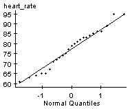
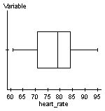
From the earlier examples, we know that the resting heart rates could come from a normally distributed population and there are no outliers.

normal probability plot boxplot

Step 1:
H₀: μ = 72
H₁: μ ≠ 72

Step 2: α = 0.05 (given)

Step 3: (we'll use StatCrunch)

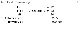
Step 4: Using StatCrunch:

StatCrunch calculations

Step 5: Since the P-value < α, we reject the null hypothesis.

Step 6: Based on these results, it would appear that there is enough evidence to support the claim that the resting heart rate for students in this class is different from the national average of 72 bpm.

Statistical Significance vs. Practical Significance

There's one last point we need to discuss in this section, and it's an important one. We need to talk about the difference between a result being statistically significant versus a result that is practically significant.

The idea is this - suppose we're comparing the performance of men and women in mathematics. To compare, we use a particular exam, given randomly to a certain number of students from across the country. We assume the difference between the two groups is zero, but we wonder whether it might be different. In that case, our null and alternative hypotheses might look something like this:

H₀: μ = 0
H₁: μ ≠ 0

Let's suppose that women are only slightly better than men on this exam - say a difference of 0.5 (if we assume the scale is 0-100). If we have a sample of 30 students - 15 men and 15 women - it'll be very hard to get a sample mean very far from zero, and so it'd be pretty rare that we'd actually find enough evidence to reject the null hypothesis (meaning we'd be making Type II error - not rejecting H₀ when we should).

On the other hand, if we had 10,000 students, it'd be very likely to get sample mean very close to the real mean, and a sample size of 10,000 would give us an extremely small P-value - definitely small enough to reject H₀.

Here's the thing - in that second case, we'd reject the null hypothesis and say that the evidence supports the claim that men and women are different, but the difference in practical terms is insignificant. So statistical significance (enough evidence to reject the null hypothesis) doesn't necessarily imply practical significance.

Beware of studies with very large sample sizes that claim statistical significance. It may be that the differences have no practical meaning.

As an illustration, check out this comic from XKCD:

XKCD comic