Section 9.2: Estimating a Population Mean
Objectives
By the end of this lesson, you will be able to...
- state properties of Student's t-distribution
- determine t-values
- construct and interpret a confidence interval for a population mean
- find the sample size needed to estimate the population mean within a given margin of error
For a quick overview of this section, watch this short video summary:
Similar to confidence intervals about proportions from Section 9.1, we can also find confidence intervals about population means. Using the same general set-up, we should have something like this:
point estimate ± margin of error
What's our point estimate for the population mean? Why, the sample mean, of course! The margin of error will be similar as well:
![]()
If you recall, we discussed the distribution of ![]() in Chapter 8:
in Chapter 8:
The Central Limit Theorem
Regardless of the distribution shape of the population, the sampling distribution of ![]() becomes approximately normal as the sample size n increases (conservatively n≥30).
becomes approximately normal as the sample size n increases (conservatively n≥30).
The Sampling Distribution of 
If a simple random sample of size n is drawn from a large population with mean μ and standard deviation σ, the sampling distribution of ![]() will have mean and standard deviation:
will have mean and standard deviation:
| and |
where ![]() is the standard error of the mean.
is the standard error of the mean.
So substituting into the above formula, we get:
![]()
There's another problem here, similar to the previous section - if we're looking for a confidence interval for the population mean, μ, how would we know σ? So like before, we can introduce an estimate there - in this case, the sample standard deviation, s. This introduces a lot of variability, though, since s can differ quite a bit from σ. As a result, we need to introduce a new distribution that's similar to the standard normal, but takes into consideration some of this variability. It's called the Student's t-Distribution.
Student's t-Distribution
The so-called Student's distribution has an interesting history. Here's a quick summary taken from Wikipedia:
The "student's" distribution was actually published in 1908 by W. S. Gosset. Gosset, however, was employed at a brewery that forbade the publication of research by its staff members. To circumvent this restriction, Gosset used the name "Student", and consequently the distribution was named "Student t-distribution".
Source: Wikipedia
Gosset was trying to do research dealing with small samples. He found that even when the standard deviation was not known, the distribution of the sample means was still symmetric and similar to the normal distribution. In fact, as the sample size increases, the distribution approaches the standard normal distribution.
Student's t-Distribution
Suppose a simple random sample size n is taken from a population. If the population follows a normal distribution, then
![]()
follows a Student's t-distribution with n-1 degrees of freedom.*
* The concept of degrees of freedom is pretty abstract. One way to think of it is like this: suppose five students are choosing from five different lollipops. Each of the first four students has a choice, but the last student does not, so there are 5-1=4 degrees of freedom.
The key idea behind the t-distribution is that it has a similar shape to the standard normal distribution, but has more variability and is affected by n.
Exploring the t-Distribution
 To do some exploring yourself, go to the Demonstrations Project from Wolfram Research, and download the Student's t-Distribution demonstration. If you haven't already, download and install the player by clicking on the image to the right.
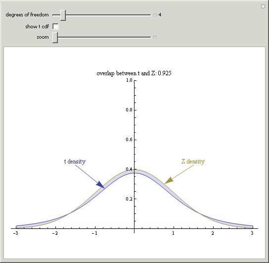
Once you have the player installed and the Student's t-Distribution demonstration downloaded, uncheck the show t-cdf box (see below) and move the slider for the degrees of freedom to see the relationship between the standard normal distribution and the t-distribution.
You should notice that as the degrees of freedom increase, the distributions become more and more similar.
Finding Critical Values
Find critical values in the t-distribution using a table will be a bit different from finding critical values for the standard normal distribution.
Before we start the section, you need a copy of the table. You can download a printable copy of this table, or use the table in the back of a textbook. It should look something like the image below (trimmed to make it more viewable).

Notice that unlike with the standard normal table, the t-table has probabilities along the top and critical values in the middle. This is because we primarily use the t-table to find tα - the value with α area (probability) to the right.
Let's try an example.
Example 1
Find t0.05 with 21 degrees of freedom. You can use the table above, or print one out yourself. Any textbook should also come with a copy you can use.

We can see form the table that t0.05 = 1.721.
Finding Critical Values Using StatCrunch
Click on Stat > Calculators > T Enter the degrees of freedom, the direction of the inequality, and the probability (leave X blank). Then press Compute. The image below shows the t-value with an area of 0.05 to the right if there are 15 degrees of freedom.
|
Example 2
Use the technology of your choice to find t0.01 with 14 degrees of freedom
t0.01, 14 ≈ 2.624
Constructing Confidence Intervals
Before we can start constructing confidence intervals, we need to review some of the theoretical framework we set up in Chapter 8. In particular, the information about the distribution of ![]() .
.
The Central Limit Theorem
Regardless of the distribution shape of the population, the sampling distribution of ![]() becomes approximately normal as the sample size n increases (conservatively n≥30).
becomes approximately normal as the sample size n increases (conservatively n≥30).
The Sampling Distribution of 
If a simple random sample of size n is drawn from a large population with mean μ and standard deviation σ, the sampling distribution of ![]() will have mean and standard deviation:
will have mean and standard deviation:
| and |
where ![]() is the standard error of the mean.
is the standard error of the mean.
Constructing a (1-α)100% Confidence Interval about μ
In general, a (1-α)100% confidence interval for μ when σ is unknown is
![]()
where ![]() is computed with n-1 degrees of freedom.
is computed with n-1 degrees of freedom.
Note: The sample size must be large (n≥30) with no outliers or the population must be normally distributed.
Example 3
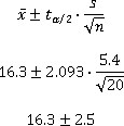
Suppose we'd like to know how many hours per week online students at ECC work. If we take a sample of 20 students and find a mean of 16.3 hours with a standard deviation of 5.4 hours, construct a 95% confidence interval for the average of all online ECC students.
Since we're looking for a 95% confidence interval, α = 0.05, so we need t0.025, 19.
Using the table or technology, we get t0.025, 19 ≈ 2.093.

So a 95% confidence interval for the number of hour worked per week by online ECC students is 13.8 to 18.8 hours.
Finding Confidence Intervals Using StatCrunch
|
Example 4
In Example 1 in Section 7.4, we looked the resting heart rates of 25 Statistics students.
| heart rate | ||||
| 61 | 63 | 64 | 65 | 65 |
| 67 | 71 | 72 | 73 | 74 |
| 75 | 77 | 79 | 80 | 81 |
| 82 | 83 | 83 | 84 | 85 |
| 86 | 86 | 89 | 95 | 95 |
(Click here to view the data in a format more easily copied.)
Use the data to construct a 90% confidence interval for the true average resting heart rate of the students in this class.
Be sure to check that the conditions for creating confidence intervals are met.
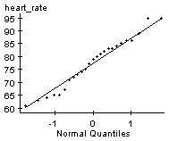
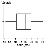
From the earlier example, we know that the resting heart rates could come from a normally distributed population and there are no outliers.


Using StatCrunch to find the confidence interval, we get the following result:

So a 90% confidence interval for the average heart rate of the students in the class is 74.1 to 80.7 bpm.
Note: This is very similar to the previous example because the standard deviation was close to the assumed value and the sample size is fairly large. It should be noted that the interval is wider, just not significantly.
Determining the Sample Size Needed
Suppose instead of trying to calculate a confidence interval given a sample mean and sample size, you are targeting a specific accuracy.
For example, say you'd like to know the average IQ of ECC students within 3 points. What sample size you would need?
The way we answer these types of questions is to go back to the margin of error definition:
The margin of error, E, in a (1-α)100% confidence interval for μ is
![]()
where n is the sample size.
If we're given the margin of error, we can solve for the sample size and get ![]() .
.
Uh-oh... another problem. How can we figure out the t-value, when we need the degrees of freedom... which depends on the sample size?! The key here is that for larger sample sizes, the t-distribution approaches the standard normal distribution (think about it - as n increases, the sample standard deviation gets closer to the population standard deviation). So what we can do instead is use z to approximate t.
The sample size required to estimate μ with a (1-α)100% level of confidence and a margin of error, E, is:
![]()
where n is rounded up to the nearest whole number.
Example 5
Let's again refer to the IQs of ECC students. How many students would we need to sample if we wanted a 95% confidence interval for the average IQ of ECC students to be within 3 points of the true population mean? (Recall that σ = 15 for IQs.)
Using the formula above, we get the following result:
![]()
This means we need at least 96.04 students, so we should sample 97.


