Section 7.2: Applications of the Normal Distribution
Objectives
By the end of this lesson, you will be able to...
- find and interpret the area under a normal curve
- find the value of a normal random variable
For a quick overview of this section, watch this short video summary:
Finding Areas Using a Table
Once we have the general idea of the Normal Distribution, the next step is to learn how to find areas under the curve. We'll learn two different ways - using a table and using technology.
Since every normally distributed random variable has a slightly different distribution shape, the only way to find areas using a table is to standardize the variable - transform our variable so it has a mean of 0 and a standard deviation of 1. How do we do that? Use the z-score!
| Z = | x - μ |
| σ |
As we noted in Section 7.1, if the random variable X has a mean μ and standard deviation σ, then transforming X using the z-score creates a random variable with mean 0 and standard deviation 1! With that in mind, we just need to learn how to find areas under the standard normal curve, which can then be applied to any normally distributed random variable.
Finding Area under the Standard Normal Curve to the Left
Before we look a few examples, we need to first see how the table works. Before we start the section, you need a copy of the table. You can download a printable copy of this table, or use the table in the back of a textbook. It should look something like this:
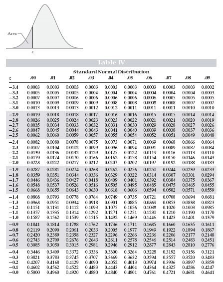
It's pretty overwhelming at first, but if you look at the picture at the top (take a minute and check it out), you can see that it is indicating the area to the left. That's the key - the values in the middle represent areas to the left of the corresponding z-value. To determine which z-value it's referring to, we look to the left to get the first two digits and above to the columns to get the hundredths value. (Z-values with more accuracy need to be rounded to the hundredths in order to use this table.)
Say we're looking for the area left of -2.84. To do that, we'd start on the -2.8 row and go across until we get to the 0.04 column. (See picture.)
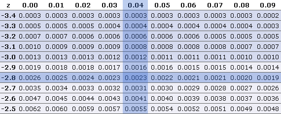
From the picture, we can see that the area left of -2.84 is 0.0023.
Finding Areas Using StatCrunch
|
Click on Stat > Calculators > Normal Enter the mean, standard deviation, x, and the direction of the inequality. Then press Compute. The image below shows P(Z < 1.23).
Note that for Z, the mean is 0 and the standard deviation is 1. |
Let's try some examples.
Example 1
a. Find the area left of Z = -0.72
The area left of -0.72 is approximately 0.2358.
b. Find the area left of Z = 1.90
The area left of 1.90 is approximately 0.9713.
Finding Area under the Standard Normal Curve to the Right

To find areas to the right, we need to remember the complement rule. Take a minute and look back at the rule from Section 5.2.
Since we know the entire area is 1,
(Area to the right of z0) = 1 - (Area to the left of z0)
Example 2
a. Find the area to the right of Z = -0.72
| area right of -0.72 | = | 1 - (the area left of -0.72) |
| = | 1 - 0.2358 | |
| = | 0.7642 |
b. Find the area to the right of Z = 2.68
| area right of 2.68 | = | 1 - (the area left of 2.68) |
| = | 1 - 0.9963 | |
| = | 0.0037 |
An alternative idea is to use the symmetric property of the normal curve. Instead of looking to the right of Z=2.68 in Example 2 above, we could have looked at the area left of -2.68. Because the curve is symmetric, those areas are the same.
Finding Area under the Standard Normal Curve Between Two Values
To find the area between two values, we think of it in two pieces. Suppose we want to find the area between Z = -2.43 and Z = 1.81.

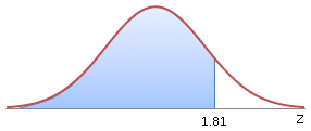
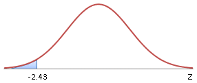
What we do instead, is find the area left of 1.81, and then subtract the area left of -2.43. Like this:
 |
| – |
 |
| = |
 |
So the area between -2.43 and 1.81 = 0.9649 - 0.0075 = 0.9574
Note: StatCrunch is able to calculate the "between" probabilities, so you won't need to perform the calculation above if you're using StatCrunch. Just use the Between option:
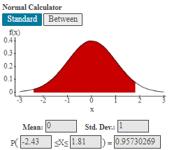
Example 3
a. Find the area between Z = 0.23 and Z = 1.64.
area between 0.23 and 1.64 = 0.9495 - 0.5910 = 0.3585
b. Find the area between Z = -3.5 and Z = -3.0.
area between -3.5 and -3.0 = 0.0013 - 0.0002 = 0.0011
Finding Areas Under a Normal Curve Using the Table
- Draw a sketch of the normal curve and shade the desired area.
- Calculate the corresponding Z-scores.
- Find the corresponding area under the standard normal curve.
If you remember, this is exactly what we saw happening in the Area of a Normal Distribution demonstration. Follow the link and explore again the relationship between the area under the standard normal curve and a non-standard normal curve.

Finding Areas Under a Normal Curve Using StatCrunch
Even though there's no "standard" in the title here, the directions are actually exactly the same as those from above!
* Note that for Z, the mean is 0 and the standard deviation is 1. |
Now we finally get to the real reason we study the normal distribution. We want to be able to answer questions about variables that are normally distributed. Questions like..
- What proportion of individuals are geniuses?
- Is a systolic blood pressure of 110 unusual?
- What percentage of a particular brand of light bulb emits between 300 and 400 lumens?
- What is the 90th percentile for the weights of 1-year-old boys?
All of these questions can be answered using the normal distribution!
Example 4
Let's consider again the distribution of IQs that we looked at in Example 1 in Section 7.1.
We saw in that example that tests for an individual's intelligence quotient (IQ) are designed to be normally distributed, with a mean of 100 and a standard deviation of 15.
We also saw that in 1916, psychologist Lewis M. Thurman set a guideline of 140 (scaled to 136 in today's tests) for "potential genius".
Using this information, what percentage of individuals are "potential geniuses"?
Solution:
- Draw a sketch of the normal curve and shade the desired area.

- Calculate the corresponding Z-scores.
Z = X - μ = 136 - 100 = 2.4 σ 15 - Find the corresponding area under the standard normal curve.
P(Z>2.4) = P(Z<-2.4) = 0.0082.
Based on this, it looks like about 0.82% of individuals can be characterized as "potential geniuses" according to Dr. Thurman's criteria.
Example 5
In Example 2 in Section 7.1, we were told that weights of 1-year-old boys are approximately normally distributed, with a mean of 22.8 lbs and a standard deviation of about 2.15. (Source: About.com)
If we randomly select a 1-year-old boy, what is the probability that he'll weigh at least 20 pounds?
Solution:
Let's do this one using technology. We should still start with a sketch:

Using StatCrunch, we get the following result:

According to these results, it looks like there's a probability of about 0.9036 that a randomly selected 1-year-old boy will weigh more than 20 lbs.
Why don't you try a couple?
Example 6
Suppose that the volume of paint in the 1-gallon paint cans produced by Acme Paint Company is approximately normally distributed with a mean of 1.04 gallons and a standard deviation of 0.023 gallons.
What is the probability that a randomly selected 1-gallon can will actually contain at least 1 gallon of paint?
In this case, we want P(X ≥ 1). Using StatCrunch again, we get the following result:

According to the calculation, it looks like the probability that a randomly selected can will have more than 1 gallon is approximately 0.9590.
Example 7
Suppose the amount of light (in lumens) emitted by a particular brand of 40W light bulbs is normally distributed with a mean of 450 lumens and a standard deviation of 20 lumens.
What percentage of bulbs emit between 425 and 475 lumens?
To answer this question, we need to know:
P(425 < X < 475)
To use StatCrunch, we'll have to find the probability of being less than 425, and then subtract that from the probability of being less than 475:
P(X<425):

P(X<475):

So P(425 < X < 475) = 0.8944 - 0.1056 = 0.7888
So the percentage emitting between 425 and 475 lumens is about 79%.
Finding Values
The next type of question comes from the other direction. Instead of giving values and asking for the probability, we'll now be looking at problems where the probability is known, but the values are not. Questions like:
- What is the 90th percentile for the weights of 1-year-old boys?
- What IQ score is below 80% of all IQ scores?
- What weight does a 1-year-old boy need to be so all but 5% of 1-year-old boys weight less than he does?
As with the previous types of problems, we'll learn how to do this using both the table and technology. Make sure you know both methods - they're both used in many fields of study!
Finding Z-Scores Using the Table
The idea here is that the values in the table represent area to the left, so if we're asked to find the value with an area of 0.02 to the left, we look for 0.02 on the inside of the table and find the corresponding Z-score.

Since we don't have an area of exactly 0.02, we have to think a bit. We have two choices: (1) take the closest area, or (2) average the two values if it's equidistant from the two areas.
In this case, it's almost equidistant, so we'll take the average and say that the Z-score corresponding to this area is the average of -2.05 and -2.06, so -2.055.
Finding Normally Distributed Values Using StatCrunch
* Note that for Z, the mean is 0 and the standard deviation is 1. |
Let's try a few!
Example 8
a. Find the Z-score with an area of 0.90 to the left.
Using the normal calculator in StatCrunch, we get the following result:

So the Z-score with an area of 0.90 to the left is 1.28. (We usually round Z-scores to the hundredths.)
b. Find the Z-score with an area of 0.10 to the right.
This is actually the same value as Example 7 above! An area of 0.10 to the right means that it must have an area of 0.90 to the left, so the answer is again 1.28.
c. Find the Z-score such that P( Z < z0 ) = 0.025.
Using StatCrunch, we get the following result:

So the Z-score is -1.96.
So we've talked about how to find a z-score given an area. If you remember, the technology instructions didn't specify that the distribution needed to be the standard normal - we actually find values in any normal distribution that correspond to a given area/probability using those same techniques.
Example 9
Referring to IQ scores again, with a mean of 100 and a standard deviation of 15. Find the 90th percentile for IQ scores.
Solution:
First, we need to translate the problem into an area or probability. In Section 3.4, we said the kth percentile of a set of data divides the lower k% of a data set from the upper (100-k)%. So the 90th percentile divides the lower 90% from the upper 10% - meaning it has about 90% below and about 10% above.
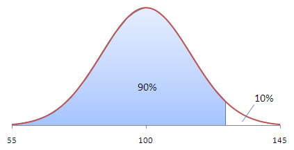
Using StatCrunch, we get the following result:
Therefore, the 90th percentile for IQ scores is about 119.
Example 10
Suppose that the volume of paint in the 1-gallon paint cans produced by Acme Paint Company is approximately normally distributed with a mean of 1.04 gallons and a standard deviation of 0.023 gallons.
What volume can the Acme Paint Company say that 95% of their cans exceed?
This would be the value with only 5% less than it. Using StatCrunch, we have the following result:

Based on this calculation, the Acme Paint Company can say that 95% of its cans contain at least 1.002 gallons of paint.
Example 11
Referring to the weights of 1-year-old boys again. (The weights of 1-year-old boys are approximately normally distributed, with a mean of 22.8 lbs and a standard deviation of about 2.15.)
What weight does a 1-year-old boy need to be so all but 5% of 1-year-old boys weight less than he does?
Using StatCrunch again, we find the value with an area of 0.95 to the left:
.jpg)
So a 1-year-old boy would need to weigh about 26.3 lbs. for all but 5% of all 1-year-old boys to weigh less than he does.
Finding zα
The notation zα ("z-alpha") is the Z-score with an area of α to the right.
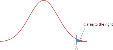
The concept of zαis used extensively throughout the remainder of the course, so it's an important one to be comfortable with. The applications won't be immediately obvious, but the essence is that we'll be looking for events that are unlikely - and so have a very small probability in the "tail".
Let's try some examples.
Example 12
a. Find z0.01
Using StatCrunch, we get the following result:

Therefore, z0.01= 2.33
b. Find z0.05
Using StatCrunch, we get the following result:

Therefore, z0.05= 1.64 (or 1.645)
c. Find z0.025
Using StatCrunch, we get the following result:

Therefore, z0.025= 1.96


