Section 5.1: Probability Rules
Objectives
By the end of this lesson, you will be able to...
- apply the rules of probability
- compute and interpret probabilities using the empirical method
- compute and interpret probabilities using the classical method
- recognize and interpret subjective probabilities
For an overview probability, watch this video:
Probability
So what is probability? Most of us already have an idea. We all know that the probability of heads when flipping a fair coin is 1/2, but what does that mean?
- One out of every two flips will be heads?
- If we have two heads in a row, the next two must be tails?
- Exactly 50 out of every 100 flips will be heads?
In fact, none of these are correct!
In general, probability is a measure of the likelihood of some outcome. We use it not to describe what will happen in one particular event, but rather, what the long-term proportion that outcome will occur.
So the key here isn't that 1 out of every 2 coin flips, or 50 out of every 100 coin flips will be heads, but that over the long term, about 1/2 will be.
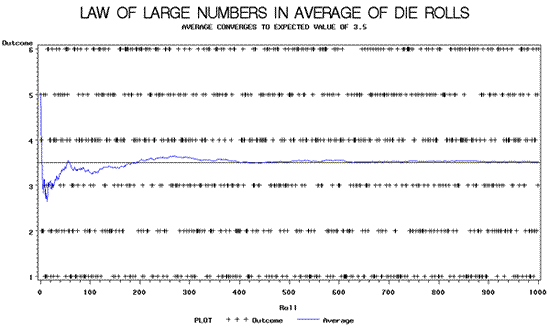
This concept is called the Law of Large Numbers. The image below is from Wikipedia, and shows the idea. It's demonstrating rolling a fair 6-sided die, and calculating the average number. We know that all 6 are equally likely, so the average should be (1+2+3+4+5+6)/6 = 3.5. From the image, we can see that while it isn't 3.5 initially, it does tend toward that as the number of rolls increases.

Note: This image is in the public domain and is copyright free.
Probability Experiments
There are some key terms we should outline before going much further.
In probability, an experiment is any process where the results are uncertain. We call the sample space, S, the collection of all possible outcomes. A probability event is any collection of outcomes from the experiment.
Example 1
Suppose we have a family with three children, and we consider the sex of those three children. If we let B represent a boy and G represent a girl, here is the sample space:
S = { BBB, BBG, BGB, GBB, BGG, GBG, GGB, GGG}
There are thus 8 outcomes in this experiment.
One possible event might be:
E = the family has exactly two girls = { BGG, GBG, GGB }
Example 2
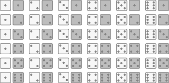
Suppose a fair six-sided die is rolled twice.
What is the sample space?
S is all possible pairs:
S = { (1,1), (1,2), (1,3), ... (6,5), (6,6) }

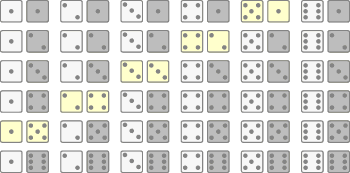
If we define the event E = the sum of the two dice is more than 10, what outcomes are in E?
E = { (5,6), (6,5), (6,6) }
Unusual Events
Suppose we consider the previous example about rolling two dice. The probability of having the sum of the two dice be more than 10 would be 3/36 or 1/12. Is this unusual? On average, it will occur about 1 in 12 times. Is that unusual enough? We have to be careful when we characterize an event as unusual.
Typically, we say that an event with a probability less than 5% is unusual, but this isn't a hard cutoff. It depends on the context.
Suppose we're planning on making a decision one way, unless the probability of a particularly "unusual" event is too high.
One example might be the jury in a capital case, punishable by death. In this example, jurors need to be sure "beyond a reasonable doubt" that the defendant is guilty. If they decide to convict if they're 95% sure, this means that the "unusual" event that they're wrong has a probability of 5%. If you're that defendant, that's definitely not "unusual" enough!
On the other hand, suppose we're planning a picnic on a nice summer day. If the risk of a rain shower isn't too high, we'll plan on the picnic. In this case, we might set our cutoff at 20% - anything less than that is too unusual (or unlikely) to happen, so we'll risk it.
Calculating Probabilities Using the Empirical Method
There are two primary methods for calculating probabilities The first is to simply look at what has happened in the past and assume the probability is the same as the relative frequency of that particular outcome. This is called the empirical probability of that event.
| P(E) ≈ relative frequency of E = | frequency of E |
| total number of trials |
Example 3
During the Spring semester of 2008, 33 out of 60 students from two sections of Mth096 Basic Algebra at ECC were successful. (Successful here is earning a C or better.)
If we define E = a Mth096 student is successful, P(E) ≈ 33/60 = 0.55.
Example 4
Suppose we give a survey to 52 Basic Algebra students, asking them to rate various statements from Strongly Agree to Strongly Disagree. If 18 of the students responded with either Agree or Strongly Agree to the statement "I enjoy math.", what is the probability that a randomly selected Basic Algebra student will enjoy math?
Since 18 out of 52 in the sample responded that way,
P(A or SA) ≈ 18/52 ≈ 0.35.
Computing Probabilities Using the Classical Method
The second primary method for calculating probabilities is the classical method. The key for this method is to assume that all outcomes are equally likely. This is how we know the probability of rolling a 6 on a fair six-sided die is 1/6, because we assume all of the outcomes (1, 2, 3, 4, 5, and 6) are equally likely.
| P(E) = | number of ways E can occur | = | N(E) |
| total number of possible outcomes | N(S) |
Example 5
Let's consider again the probability experiment from Example 2 - rolling two fair six-sided dice.
Let the event E = the sum of the two dice is 6.

Find P(E).
Since there are five ways to get a sum of 6,
P(E) = 5/36 ≈ 0.14

