Section 4.3: Diagnostics on the Least-Squares Regression Line
Objectives
By the end of this lesson, you will be able to...
- compute and interpret the coefficient of determination
- perform residual analysis on a regression model
- determine if a linear regression model is appropriate
- identify influential observations
For a quick overview of this section, watch this short video summary:
Before we can go on, we need to first determine two things:
- Does our model do a good job of predicting the results?
- Is a linear model appropriate?
We'll have two key factors to help us answer these questions. The first is called the coefficient of determination.
The Coefficient of Determination
The coefficient of determination, R2, is the percent of the variation in the response variable (y) that can be explained by the least-squares regression line.
Looking at the definition, we can see that a higher R2 is better - the LSR line does a better job of explaining the variation in the response variable.
If you'd like to, you can view the derivation on this page from Wikipedia. (Not that Wikipedia is a perfect source, but this particular page is accurate.)
Here's the end result, which shouldn't come as too much of a surprise:
R2 = r2
Here are some examples:
 |
 |
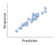
| R2 = 92.1% | R2 = 70.0% |
 |
 |
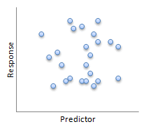
| R2 = 53.4% | No R2 = 13.5% |
The second step in residual analysis is using the residuals to determine if a linear model is appropriate. We do this by creating residual plots. A residual plot is a scatter diagram with the predictor as the x and the corresponding residual as the y.

In general, there are three things to watch out for in a residual plot:
- a pattern in the residuals
- increasing or decreasing spread
- influential observations
Patterned Residuals
If a residual plot shows a discernable pattern (like a curve), then the predictor and response variables may not be linearly related.
 |
 |
| The LSR line clearly does not fit. | The residuals show an obvious pattern. |
Increasing or Decreasing Spread
If a residual plot shows the spread increasing or decreasing, then a strict requirement of the linear model is related. (This strict requirement is called constant error variance - the error must be evenly spread.)
 |
 |
| The LSR line seems to be a great fit. | The residuals start very small, but increase as the predictor variable increases - this model does not have constant error variance. |
Outliers and Influential Observations
The next point we need to consider is the existence of outliers and influential observations. We can think of an outlier as an observation that doesn't seem to fit the rest of the data. Influential observations are similar, but with the added quality that their existence significantly affects the slope and/or y-intercept of the line.
Consider the scatter diagram shown below, along with its corresponding residual plot:
 |
 |
Let's consider the three cases indicated.
Case 1:
This case is considered an outlier because it's x-value is much lower than all but one of the other observations. To determine if it's an influential observation, we'll need to recalculate the LSR line without that observation included. Here are the results:
 |
 |
We can see that while there are some changes in the slope and y-intercept, both are reasonably similar to what they were with Case 1 included. In this case, we would describe Case 1 as an outlier, but not an influential observation.
An interesting point to note, though, is the decreased R2 value. The implication is that Case 1 actually strengthened the correlation. Think of that point pulling the line "tighter".
Case 2:
Looking back at the original diagram, it seems as though Case 2 should be influential, because there are not many values near it to minimize its effect on the LSR line. Here's the output from computer software:
 |
 |
Here we can clearly see that both the slope and y-intercept (as well as R2) are significantly different, so we would definitely characterize Case 2 as an influential observation.
Case 3:
Unlike in Case 2, this particular observation has others near it to minimize its effect, so it most likely will not be influential. Here's the output from computer software:
 |
 |
Comparing those to the original values, we can indeed see that the slope and y-intercept are both relatively similar. So while this value is an outlier (as seen very clearly on the earlier residual plot), it is not influential.
If you find your data contain outliers or influential observations, and those observations cannot be removed (because they are due to data entry errors or similar) you have only a couple options. The primary option is to collect more data to minimize their impact. The second is to use analysis methods that minimize the effect of outliers. Unfortunately, those techniques are fairly advanced and outside the scope of this course.
When a Linear Model is Appropriate
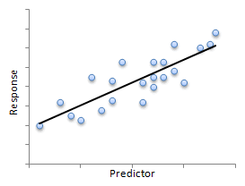
Sometimes it can be difficult to determine if any of the three above conditions have been violated, but here's a good example of a situation where a linear model does seem appropriate.
 |
 |
| The LSR line seems to fit the data. | The residuals are evenly spread above and below zero, there is no discernable pattern, and there are no outliers. |
Technology
Here's a quick overview of how to create a residual plot in StatCrunch.
Press the > on the bottom right to see any additional output. |
