Challenge Yourself
Pivot tables are a very useful feature of Excel, especially when you have a lot of data. A pivot table allows you to view the data from different perspectives. The best way for you to get the feel for what a pivot table can do for you is to play with them. So open the Pivot Table Data spreadsheet in the labs folder of my instructor folder.
To create a Pivot table, select the Insert ribbon, select the data range (or a single cell in the table Excel will suggest the entire table as the data range) on your spreadsheet, then choose Pivot Table on the left side of the ribbon.

You can choose to put the Pivot table on the same sheet as the data or on a sheet of its own.
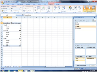
In the pane on the right, you will choose what fields you want to view. Choose Who and What. Drag the Amount field into the ∑ Value area on the bottom of the pane. This will allow you to see how much each person spent and what they spent it on. Notice that you can filter either the who and/or what to specific people or items by clicking on the arrow next to the field in the pane.

Try to figure out how to get averages instead of sums. Play with the Pivot Table to get a feel for what you can do with it.