Now that we have added all of the information to the spreadsheet we need to format it.

The first thing we need to do is format the header.  Click on cell A1,  Go to the Home tab.  In the formatting toolbar select Arial from the font list, select 16 point from the font size list and click on the bold button,

The formatting tool bar should look like the one at the right

Move to the center of the A1 cell and drag out to the F1 cell  to select all of the cells (make sure you do not select the copy cell button.

Find the Merge and Center button on the formatting tool bar and click on it.

The first line should look like the one below.

Do the same thing with the second line of text only make the font size 14.  The two lines should look like the one below.

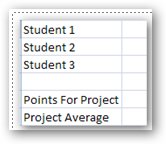
We need to make the first column larger so that we can read all of the words.  

Move the cursor on the line between the A and B cell at the top of the spreadsheet, you will see the double headed cursor appear like example at right.

Drag the column divider to the right until all of the words are present in all of the cells.  The A column should look like the one to the right.

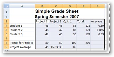
We should center all of the information between the B3 and F9 cell. To do this click on the B3 cell and with you cursor in the center of the cell drag to the F9 cell.  The Spreadsheet should look like the one below.

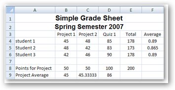
Click on the center button on the formatting tool bar.   Click on a cell outside the blue area. Your spreadsheet will look like the one below.

The last thing we need to do is reduce all of the number to two decimal places.  To do this click on cell B9 and select cells B10 and B11

Right click on the selected boxes  The list at the right will appear.  Click on Format Cells

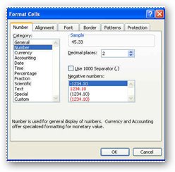
The Format Cell dialog box will appear

Make sure that the Number tab is selected.  

From the list click on Number.  

In the Decimal place box make sure 2 is selected and click on OK.

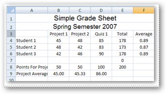
Your finished spreadsheet should look like the one below.